How hard is to find exoplanet atmospheres?

Posted on August 17, 2014 by Néstor

Introduction

I just joined a competition called ‘Three Minute Thesis’ at my university, in which I have to explain, in three minutes, what my thesis is about*. The thing is that my thesis is about detecting exoplanet (that is, planets outside our solar system) atmospheres from the ground through an effect called transmission spectroscopy but, although that sounds cool for most people (except when I mention ‘transmission spectroscopy’, which sounds like a magical, frightening and strange word for non-astronomers), I don’t really know if they understand how hard this stuff is to do. In order to show this, I want to share a little order-of-magnitude calculation that I did in order to show how hard it is to find exoplanet atmospheres through this method.

What is transmission spectroscopy?

As of today, most exoplanets discovered so far have been discovered through the method of transits: the apparent decrease in flux of a star due to a planet passing in front of it. This is, of course, a lucky event: for earth-like planets (that is, planets orbiting Sun-like stars at the same distance as the Earth), assuming orbits around stars are totally random, the probability of finding a transiting planet is $\sim 0.5\%$ ! When we are lucky enough to see this event, we can exploit a lot of information concerning the atmosphere of the planet. The effect I’m going to talk about in this post comes from a very simple idea: during a transit, part of the light gets blocked by the planet passing in front of the star but some of it also goes through the atmosphere, so the informatlon regarding the atmosphere gets imprinted on the stellar light that we receive at Earth. This is why the effect is termed transmission spectroscopy; stellar light gets transmitted through the atmosphere of the planet, and we try to detect that signature. A picture is worth more than a thousand words, so here’s a diagram I made:

Diagram showing how light is not only blocked by a transiting planet during a transit event, but also how the atmospheric signature (red ring around the blue planet) is imprinted on the stellar light. Credits: Néstor Espinoza.

Seems like a cool effect, huh? It also seems like a very small effect. Let’s first explore how small of an effect a transiting planet makes and, then, jump into the very small effect the atmosphere might be able to produce!

The tiny effect of transits

Let’s consider a planet of radius $R_p$ transiting a star of radius $R_*$ . In the absence of an atmosphere, during a transit, a planet would imprint a decrease in the observed stellar flux (energy per unit time per unit area) at first order (and assuming an orbit very close to the star) equal to the ratio of the observed areas, i.e., $\delta_\textnormal{p} = (R_p/R_*)^2$ . How small is this effect? For the case of a Jupiter-sized planet transiting a star like the Sun (where the ratio of radii is $R_p/R_*\sim 1/10$ ), $\delta \sim 1/100$ , or 1% of the stellar flux! To have an idea of how small this is, let’s first try to understand how dim a star is as seen from Earth. Consider a star like the sun at 4 lightyears away (the distance to the Alpha Centauri system for which, to date, no transiting planet has been detected) with a transiting planet like Jupiter. If we consider its luminosity to be solar, i.e. $L_\textnormal{sun}\approx 4\times 10^{26}\ \textnormal{W}$ , the observed flux at Earth of this star would be

$F_\textnormal{obs}=L_\textnormal{sun}/4\pi d^2\approx 2\times 10^{-8}\ \textnormal{W/m}^2$ .

To compare this flux, let’s consider a lightbulb, which at best has an output of around 100 W. In order to observe a similar flux as that of the star mentioned before, you would need to be at a distance

$d = \sqrt{L_\textnormal{lightbulb}/4\pi F_\textnormal{obs}}\sim 20\ \textnormal{km}$

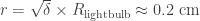
from it. For the ones out there that have come to Santiago de Chile, this distance is roughly the distance from the top of San Cristobal hill to the farthest lightbulb you can see. This photo might enlighten your imagination:

Santiago de Chile as seen from San Cristóbal hill. Credits: Aldo Felipe Paez.

Pretty dim, huh? Now, how small is the effect of a 1% decrease in flux due to a transiting planet? Well, remember that a 1% decrease in flux for a star’s flux happens when a planet 1/10 of its radius passes in front of it when the star is like our Sun. The farthest lightbulb you can see in the photo comes from a source with a radius not bigger than, say, ~10 cm; a 1% decrease in flux in that lightbub then can arise from an object 1/10 of its size passing in front of it, or, an object with a radius of ~1 cm! That’s like detecting the effect of a moth passing between you and that lightbulb very close to it! That is a really small effect. However, as I mentioned in the introduction, most planets have been detected in this way, and there are large collaborations of astronomers trying to detect more exoplanets like these ones (have you ever heard of HATSouth, for example?). We might say that this is one of the most successful exoplanet finding tools to date! Now, If you think the effect of transits is small, wait until you see the really, really small effect that the atmosphere imprints on exoplanetary transits.

The (really) tiny effect of transmission spectroscopy

Let’s consider the same planet as before, but let’s now assume that it has an atmosphere. The effect that one usually wants to detect is the absorption feature of some atomic and/or molecular feature and, therefore, what one usually seeks is a transit event observed in different wavelengths. If there is absorption in a given wavelength, then the planet will look bigger than in other wavelengths. To simplify the matters, let’s assume that the whole atmosphere is of this given element that absorbs all the light at a given wavelength. If we assume that the only force that keeps this element from escaping to outer space is gravity, then it should be a given height where gravity is so small that the element can escape due to the internal kinetic energy of the compound. If the kinetic energy is of the same order of magnitude as the gravitational potential, then the gas will start escaping from the atmosphere. Assuming the element behaves more or less like an ideal gas and is more or less isothermal, the mean kinetic energy of it is given by

$E_\textnormal{K}\sim k_BT,$

where $k_B\approx 1.4\times10^{-23}\ \textnormal{J/K}$ is Boltzmann’s constant and $T$ is the temperature of the gas in Kelvins. On the other hand, if the element has a mass $m$ , the graviational potential is given by

$E_\textnormal{g}\sim mgh,$

where $g$ is the gravitational acceleration of the planet and $h$ is the height at which this potential is measured. Now, when $E_\textnormal{K}\sim E_\textnormal{g}$ , the kinetic energy is enough to let some of the element escape to outer space. This occurs at a height

$H\sim k_BT/mg.$

This number is usually known as the scale height, and it defines a characteristic height to a given atmosphere (its actually the height at which an atmosphere in thermodynamic and hydrostatic equilibrium decreases its presure by a factor $e\sim 3$ ). For Earth, for example, $g\approx 10\ \textnormal{m/s}^2$ , $T\sim 300$ K and the mean mass of the constituents is $m\approx 29m_p$ , where $m_p\approx 2\times 10^{-27}\ \textnormal{kg}$ is the mass of a proton. This gives

$H_\textnormal{Earth}\sim 5\ \textnormal{km},$

which is the characteristic height of our atmosphere. Of course, this is not the height of the whole atmosphere that would be probed by the effect of transmission spectroscopy; this largely depends on the constituents, layers and properties of those layers in each atmosphere (i.e., the pressure-temperature profile). As a good average between thin ( $H$ ) and very extended ( $10H$ ) atmospheres, $\sim 5H$ seem to be a reasonable choice. Let’s now assume then that our close-in Jupiter transiting planet has an atmosphere with a height of $5H$ . Most of the close-in Jupiters have been discovered at periods around $3$ days, which implies temperatures close to $\sim 2000$ K, reason by which these planets are usually called “hot” Jupiters. If we assume it to be an almost exact Jupiter analog, its gravity should be $g=GM/R^2\sim 30\ \textnormal{m/s}^2$ . Furthermore, it should be made mainly of hydrogen gas, just as Jupiter, so $m\approx 2m_p\sim 4\times 10^{-27}\ \textnormal{kg}$ . Combining all of that information, the scale-height for our Hot Jupiter should be

$H_\textnormal{HJ}\sim 200\ \textnormal{km}.$

In this case then, if the atmosphere were to absorb all the light at a given wavelength, the planet would appear to have a radius of $R_{\textnormal{p+atm}}=R_p+5H_{\textnormal{HJ}}$ . This induces a transit signal equal to the ratios of the areas, but now with the “new” planet + atmosphere radius,

$\delta_\textnormal{p+atm}=(R_{\textnormal{p+atm}}/R_*)^2 = \delta_\textnormal{p}+(10R_pH_{\textnormal{HJ}}+25H_{\textnormal{HJ}}^2)/R_*^2\approx\delta_\textnormal{p}+10R_pH_{\textnormal{HJ}}/R_*^2,$

or, in a more compact form,

$\delta_\textnormal{p+atm}\approx\delta_\textnormal{p}+\delta_{\textnormal{atm}},$

where we have ommited the $25H_{\textnormal{HJ}}^2/R_*^2$ term (its very small compared to the other terms), used the term $\delta_p = (R_p/R_*)^2$ already shown before and defined the term $\delta_{atm}=10R_pH_{\textnormal{HJ}}/R_*^2$ . Note that is this last term that is added to the “normal” transit signal ( $\delta_p$ ), so we can interpret it also as a percentage change in flux due solely to the atmosphere. Using the radius of Jupiter to be $R_p\approx 7\times 10^4\ \textnormal{km}$ , a radius of the Sun of $R_*\approx 7\times 10^{5}\ \textnormal{km}$ and the calculated scale-height, we obtain,

$\delta_{atm} \approx 3\times 10^{-4},$

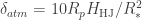
or 0.03%! That’s two orders of magnitude smaller than the transit signal $\delta_{\textnormal{p}}$ which was 1%! If we go back to our example of the lightbulb again, recalling that a change in flux of $\delta$ can arise from the ratio of the areas of the two objects, if our lightbulb has a $R_\textnormal{lightbulb}=10\ \textnormal{cm}$ radius, then a change in flux of $\delta = 3\times 10^{-4}$ can come from an object of size

$r = \sqrt{\delta}\times R_\textnormal{lightbulb}\approx 0.2\ \textnormal{cm}$

passing close-by, in front and between us and the lightbulb. That’s measuring the effect of a 2 mm object passing in front of the lightbulb! Enough precision to give the moth a coat for the winter or a bathing suit for the summer! Despite the effect being very small, this effect has been measured successfully both from space and ground based observatories. However, these studies have been done only for a handful of systems; there are many more problems than just getting enough light from the stars in order to detect this effect, where ground based observations are by far the most challenging ones. Imagine trying to measure that 0.03% flux change from the lightbulb, but with fog, while your instrument moves, rotates and shakes due to its own gravity…those systematic effects are the biggest problems in current ground-based measurements. It’s quite a challenge, and that’s actually what makes it so interesting! Frontier science usually comes from beating those challenges with clever ideas so, stay tuned!

Conclusions

Detecting exoplanet atmospheres is hard. Very hard. In the best-case scenario, It is analogous to trying to measure the flux change in a lightbulb 20 km away from your location with enough precision to build a coat or a swimsuit for a moth passing in front and very close to the lightbulb. The signal depends largely on temperature, gravity and the mass of the elements in the atmosphere; it favours higher temperatures, lower gravities and lighter constituents. The biggest challenge, though, is not the signal but the actual systematic effects the instruments and the Earth’s atmosphere (for the case of ground-based observations) imprints on the signals but various groups of astronomers are working on this as we speak…stay tuned for future discoveries!

*: As an update on this, I won the People’s Choice award in the competition! It was really cool, specially because there was no people from my department in the audience (who were the ones who voted for me).

A python with a long memory: fitting 1/f noise with PyMC

Posted on July 14, 2014 by Néstor

Introduction

Since ancient times, astronomy has been observing long-memory processes (i.e., short frequency noise) all over the place. The problem has been a tough one for lots of people working on time-series, specially for the ones involved in exoplanets, as the lightcurves (which show an apparent decrease in the observed flux of the star as the result of the planet eclipsing the star) usually show signs of red noise which can’t be neglected, as they affect the physical properties of the planet and the star derived from these measurements (Pont, Zucker & Queloz, 2006).

A special case of these kinds of long-memory processes, flicker (or 1/f, or pink) noise, has attracted the attention of the community in general for more than forty years (see, e.g., Press, 1978) but, until recent years, little work has been done to account for that kind of noise, despite the fact that approximate solutions for the problem have been around since almost twenty years (Wornell, 1995). However, a few years ago, Carter & Winn (2009) published a very interesting paper in which they derive and implement a very interesting methodology following the approaches given in Wornell (1995), in which a wavelet-based approach is used to transform the time series. The trick is that in wavelet space, 1/f processes have nearly diagonal covariance matrices, so the problem is extremly simplified when wavelet-transforming the time-series. The implementation assumes a model of the form:

$f(t,\theta) + \epsilon_{\textnormal{1/f}}(t)+\epsilon_{\textnormal{wn}}(t),$

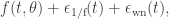
where the first term is a deterministic model with parameters $\theta$ , the second term is a zero mean 1/f stochastic process (which is defined by only one parameter, $\sigma_r$ , which defines its amplitude but is not the square root of its variance), implying its Power Spectral Density is proportional to $1/f$ and the third term is a zero mean white noise process, here assumed to be gaussian (and hence with only one parameter defining it, $\sigma_w$ , the square root of its variance). Furthermore, the model assumes the time-sampling is uniform.

The work of Carter & Winn (2009) was implemented in a code called Transit Analysis Package (TAP; Gazack et al., 2012), which was coded in Interactive Data Language (IDL), a very nice coding plataform/language, but also a very expensive one for a poor graduate student like myself¹. So I decided to make my own implementation in Python of the work of Carter & Winn (2009), but using PyMC, a really amazing python module that implements Bayesian statistical models and fitting algorithms, which includes Markov chain Monte Carlo. In this blog post I want to make a little tutorial on how to use this implementation; you can download all the codes for your research in my personal webpage [here]. If you use it, please, cite the work of Carter & Winn (2009) and acknowledge the hard work I have put in this implementation.

Installing the package

To install this package, download the code from my the package repository, and unpack it to a folder. Inside you will find a install.py file that you have to run, and this will create a file called FWT.so inside the WaveletCode folder; this is a Discrete Wavelet Transform and Inverse Wavelet Transform implementation in C that I wrote, based on the algorithm in the Numerical Recipes. The coding in C is done mainly because it is fast, and it can be called from Python as you can check on the Wavelets.py code in that same folder.

After the above is done you are done! From now on, I will assume you are working on the same directory as the FlickerLikelihood.py file that we will use (which is on the same folder as the install.py file). Let’s make a little experiment now!

A simple problem: fitting a line with 1/f + white gaussian noise

Let’s solve the simple problem of fitting a line of the form $f(t)=at+b$ which has both additive white and 1/f noise. In the following plot, I have created 1/f noise following the method of Paul Burke, with $\beta=1$ (in red), and I added white gaussian noise in order to make the problem even more challenging (black dots):

The next step is to add a model to that noise. I added a model of the form $f(t)=at+b$ , with $a=0.5$ and $b=3$ , which is plotted in the following figure (you can download the dataset from here to run the codes showed here):

And now comes the code. Using the FlickerLikelihood.py file contained in the package, which calculates the likelihood derived by Carter & Winn (2009) with the function get_likelihood, which takes as inputs (1) the residuals, (2) the standard deviation of the white noise, $\sigma_w$ and (3) a parameter that defines the amplitude of the flicker noise model, $\sigma_r$ , one can create a likelihood using our model with PyMC, which I called LineFlickerModel.py:

import sys
sys.path.append("WaveletCode")
import FlickerLikelihood
import numpy as np
from pymc import *
import Wavelets

#  Functions  #
def model(t,a,b):
    return a*t+b

# Get the data #

t,data = np.loadtxt('flicker_dataset.dat',unpack=True)

# Priors #

b = Uniform('b',-10,10)
a = Uniform('a',-1,1)
sigma_w = Uniform('sigma_w',0,100)
sigma_r = Uniform('sigma_r',0,100)

# Likelihood #
@observed
def likelihood(value=data,t=t,a=a,b=b,sigma_w=sigma_w,sigma_r=sigma_r):
    residuals=data-model(t,a,b)
    return FlickerLikelihood.get_likelihood(residuals,sigma_w,sigma_r)

With this code, now I can run some MCMC links using PyMC; the following code uses the above code and draws samples from it:

import numpy as np
import matplotlib.pyplot as plt
import pymc
import LineFlickerModel

# Set the number of iterations and burnins:
niterations = 1e5
nburn = 1e4

# Set MAP estimates as starting point of MCMC. First, calculate MAP estimates:
M = pymc.MAP(LineFlickerModel)
M.fit()
# Now set this as starting point for the MCMC:
mc=pymc.MCMC(M.variables)

# And start the sample!
mc.sample(iter=niterations+nburn,burn=nburn)

# Plot the final samples (posterior samples):
pymc.Matplot.plot(mc)
plt.show()

The results you will get will be the posterior samples for each parameter. In particular, for the fitted parameters I get:

$a=0.501 \pm 0.008$

$b=3.04 \pm 2.8$

(Here I cited the standard deviations of the posterior samples as errors). Note the huge errorbar on $b$ : this is good! It is good because due to the correlated noise, we are very uncertain about the value (recall that the 1/f noise + white gaussian noise is a stochastic process and, as such, we only observe one realization of it; we can take into account this, but this won’t make our measurements more precise, only more accurate). What if we try fitting a white gaussian noise model (as most people would do!), not taking into account that we have correlated noise? I will leave that problem to the reader, but the MCMC samples of both, the gaussian white noise run (black points) and the 1/f + gaussian white noise run (red points), are plotted on the following figure:

The results I get for the parameters are:

$a_{\textnormal{g}}=0.493 \pm 0.002$

$b_{\textnormal{g}}=4.56 \pm 0.63$

Note the very little errorbar on the estimated parameter $b_{\textnormal{g}}$ ! This is BAD! What this shows (and you can generate more datasets and simulate this claim; which is actually something Carter & Winn (2009) already did) is that, in general, the errorbars on the parameters will be more realistic if you take into account the proper noise model: on average you will get the same results, but for a particular dataset, the errorbars taking into account the 1/f noise model will be more realistic than the ones you would get by assuming a gaussian (or any) white noise model. For the statisticians on the crowd: the estimator taking into account the 1/f noise has a lower variance than the estimator taking into account white gaussian noise.

The challenge in real life is, of course, to know a-priori what kind of noise you actually have. There are several tools for this that are out of the scope of this blog post but, if you are really interested, you can check some of them on our work on this subject on Jordán, Espinoza, et. al (2013); the paper is a little technical in general, but the relevant section to this problem is Section 4.2.

Conclusions

I want to make the conclusions super short (because this was intended only as a tutorial on how to use my code), but in summary what I want to say is:

Know your noise (or at least try to understand it).
This is the best advice I can give to anyone around the world: small errorbars don’t imply high accuracy.

This is it! If you have any questions, remarks, thanks or find any bugs, please, the comment section is open! All the codes used in this example are on the GitHub repository of this package here: https://github.com/nespinoza/flicker-noise/tree/master/example.

¹: To be fair, the real reasons of why I wanted to make a Python implementation were that: (1) I stopped coding in IDL as soon as I knew Python existed, (2) most of my colleagues work in python and (3) I really wanted to make use of PyMC for this kind of analyses.

Defining which process goes to which core

Posted on March 14, 2013 by Néstor

Lately I’ve been working on really computer expensive processes which need to be run on different cores in order to obtain the results in publishing-human scale (~1 week). So far I’ve been just running the codes in terminal, but today I discovered that you can actually choose to what processor each code goes with a simple command!

Let’s suppose you have a process in a python code, say, myprocess.py, and want to run it on core X. Then, in a terminal, you do:

taskset -c X python myprocess.py

Now, the thing is to know which of the cores is busy with something, in order to run the process in other core. I’ve just installed the sysstats package (apt-get install sysstats) which, once installed, enables you to run the mpstat process, which is very helpful. You run it by doing

mpstat -P ALL 1

And this will give you something like this every second (change the “1” after ALL to “2” if you want to obtain results every 2 seconds, etc.):

01:25:27 PM  CPU    %usr   %nice    %sys %iowait    %irq   %soft  %steal  %guest   %idle
01:25:28 PM  all   21.09    0.00    0.05    0.00    0.00    0.00    0.00    0.00   78.86
01:25:28 PM    0    0.00    0.00    0.00    0.00    0.00    0.00    0.00    0.00  100.00
01:25:28 PM    1    0.00    0.00    0.00    0.00    0.00    0.00    0.00    0.00  100.00
01:25:28 PM    2    0.00    0.00    0.00    0.00    0.00    0.00    0.00    0.00  100.00
01:25:28 PM    3  100.00    0.00    0.00    0.00    0.00    0.00    0.00    0.00    0.00
01:25:28 PM    4  100.00    0.00    0.00    0.00    0.00    0.00    0.00    0.00    0.00
01:25:28 PM    5  100.00    0.00    0.00    0.00    0.00    0.00    0.00    0.00    0.00
01:25:28 PM    6  100.00    0.00    0.00    0.00    0.00    0.00    0.00    0.00    0.00
01:25:28 PM    7    0.00    0.00    0.00    0.00    0.00    0.00    0.00    0.00  100.00
01:25:28 PM    8    0.00    0.00    0.00    0.00    0.00    0.00    0.00    0.00  100.00
01:25:28 PM    9    0.00    0.00    0.00    0.00    0.00    0.00    0.00    0.00    0.00
01:25:28 PM   10    0.00    0.00    0.99    0.00    0.00    0.00    0.00    0.00   99.01
01:25:28 PM   11    0.00    0.00    0.00    0.00    0.00    0.00    0.00    0.00    0.00
01:25:28 PM   12    0.00    0.00    0.00    0.00    0.00    0.00    0.00    0.00    0.00
01:25:28 PM   13    0.00    0.00    0.00    0.00    0.00    0.00    0.00    0.00    0.00
01:25:28 PM   14    0.00    0.00    0.00    0.00    0.00    0.00    0.00    0.00    0.00
01:25:28 PM   15    0.00    0.00    0.00    0.00    0.00    0.00    0.00    0.00    0.00

To check what everything means, go to the mpstat description, but basically the number below %usr this tells you which of the cores is being used and which is not (be aware that this shows both, virtual and physical cores). Currently, I’m only using CPU 3,4,5 and 6, which have python codes running on them.

Let’s awaken core number 2 so you can see the difference with mpstat (note that I have two terminal windows open: one with mpstat running and one which will run the python code that I’m going to execute in core number 1). I have the following code, named test.py:

import numpy as np
x = 0.0
n = 1000000
for i in range(n):
    x = x+np.double(i)
print x/np.double(n)

which just takes the mean of the first n numbers. Then, I run it on core 1 by doing:

taskset -c 1 python test.py

And the output of mpstat is:

01:26:27 PM  CPU    %usr   %nice    %sys %iowait    %irq   %soft  %steal  %guest   %idle
01:26:28 PM  all   21.09    0.00    0.05    0.00    0.00    0.00    0.00    0.00   78.86
01:26:28 PM    0    0.00    0.00    0.00    0.00    0.00    0.00    0.00    0.00  100.00
01:26:28 PM    1   41.12    0.00    0.00    0.00    0.00    0.00    0.00    0.00  100.00
01:26:28 PM    2    0.00    0.00    0.00    0.00    0.00    0.00    0.00    0.00  100.00
01:26:28 PM    3  100.00    0.00    0.00    0.00    0.00    0.00    0.00    0.00    0.00
01:26:28 PM    4  100.00    0.00    0.00    0.00    0.00    0.00    0.00    0.00    0.00
01:26:28 PM    5  100.00    0.00    0.00    0.00    0.00    0.00    0.00    0.00    0.00
01:26:28 PM    6  100.00    0.00    0.00    0.00    0.00    0.00    0.00    0.00    0.00
01:26:28 PM    7    0.00    0.00    0.00    0.00    0.00    0.00    0.00    0.00  100.00
01:26:28 PM    8    0.00    0.00    0.00    0.00    0.00    0.00    0.00    0.00  100.00
01:26:28 PM    9    0.00    0.00    0.00    0.00    0.00    0.00    0.00    0.00    0.00
01:26:28 PM   10    0.00    0.00    0.99    0.00    0.00    0.00    0.00    0.00   99.01
01:26:28 PM   11    0.00    0.00    0.00    0.00    0.00    0.00    0.00    0.00    0.00
01:26:28 PM   12    0.00    0.00    0.00    0.00    0.00    0.00    0.00    0.00    0.00
01:26:28 PM   13    0.00    0.00    0.00    0.00    0.00    0.00    0.00    0.00    0.00
01:26:28 PM   14    0.00    0.00    0.00    0.00    0.00    0.00    0.00    0.00    0.00
01:26:28 PM   15    0.00    0.00    0.00    0.00    0.00    0.00    0.00    0.00    0.00

See the change in %usr on core 1 from 0.00 to 41.12? Core 1 has been awakened!

Higgs boson “discovery” and how to NOT interpret p-values

Posted on July 4, 2012 by Néstor

July 4th was an amazing day for science: a candidate for the realization of a field (well, the quantum fluctuation of it) – known as the Higgs field – could be detected: the Higgs boson. The importance of the Higgs field is enormous: it is the responsible of giving mass to everything we see around! From galaxies, stars, planets, us, atoms, etc.

If you are really interested on the physics of this mechanism, you can search around the CERN official webpage for info. I’m not talking here about the details of the physics (which, to be sincere, I don’t entirely understand) of the mechanism and the interpretations, but a little about the details of the detection and a common misinterpretation of it that I’ve seen (and heard) around.

The thing is that physicists at CERN don’t actually “see” the Higgs boson; they see the decays of it (i.e., the transformation of the energy of the boson into other different particles). Almost all particles decay in some form (and most of them very rapidly, like the Higgs!). Perhaps the most common decay is the one of Carbon-14, which allows us to estimate the age of different materials that contain carbon trough radicarbon dating. As Carbon-14, the Higgs decays in various forms but the most important ones that were detected at CERN were two: it’s decay into two photons and it’s decay into four leptons.

The analysis from there is “simple” (I’m obviously skipping some details, but this is just to have a big picture of the process). Protons collide at the LHC, and the resultant energy transforms into different particles. So if the Higgs is among those particles, it has to decay into different other particles; let’s analyse the photon-photon decay. From all the Higgs bosons that appear at the collision, a number of them decay into two photons, were the sum of the energy of the two has a definite value: the one that corresponds to the Higgs mass (energy conservation!). So in every multiple collision at the LHC, you take all photons and you pair them up. For example, if you see 3 photons, you sum the energies of the first to the second and have a pair, the second to the third and have another pair, etc. The people at CMS did this and found the following plot:

Here the y-axis is the number of (weighted) events (i.e. a measure of how many pairs with a given energy you saw), and the x-axis shows the energy of the sum of the photons (a direct measure of the mass of the particle). The dotted line is the model without the Higgs boson and the red line is the model with the Higgs boson: apparently the model with the Higgs fits pretty well!

So far so good. However, here comes the misinterpretation of the results: from all of the above, physicists calculate what is called a (local) p-value, to measure the significance of the “bump” that we’ve seen on the plot above. For anyone who hasn’t taken any statistic courses, the p-value is the the probability of observing data at least as extreme as that observed, given that the null hypothesis is true. I must be clear with this definition, and to be clear, what better than an example? Imagine I have a coin and I throw it twenty times, with the following results (H: heads, T: tails):

T H H H H H H H H H H H H T H T H H H H.

I now ask you: do you think the coin is unbiased? Your answer would probably be no (there are clearly more heads than tails!). Now I ask you again…why? You might reply that, given that the coin is unbiased, the results that I showed to you are very unlikely, so you’ll probably reject the hypothesis that the coin is unbiased. The p-value serves for doing this in a more “orthodox” way: you choose a null hypothesis, $H_0$ (in this case $H_0$ : “the coin is unbiased”), an alternative hypothesis, $H_1$ (in this case $H_1$ : “the coin is biased”), and you calculate the probability of observing data at least as extreme as that observed, given that the null hypothesis is true (in our case the probability of observing data as least as extreme as that observed, “given that the coin is unbiased”). If this probability is low enough ^[1] (i.e., if given the null hypothesis $H_0$ : “the coin is unbiased”, the probability of observing data at least as extreme as mine is apparently low, which is our case, i.e., it is unlikely to observe our data or more extreme combinations of head and tails given that the coin is unbiased), then you usually reject the null hypothesis (which was our case: we rejected the hypothesis $H_0$ : “the coin is unbiased”). If the probability is not low enough, you usually can’t say anything, so you fail to reject the null hypothesis. I’ll warn you to be very careful with these statements: rejecting the hypothesis is not the same as proving it wrong. The results of the coin that I showed could come in fact from an unbiased coin, however, among all the possible combinations of heads and tails after twenty throws, it is very unlikely to obtain the data that we saw: this is what a significance test helps you decide. In the same way, failing to reject the null hypothesis is not the same as proving the null hypothesis.

I’m going to be pretty hard on the above definition: the p-value IS NOT the probability of the coin being unbiased. Please save this in your mind:

$P(H_0)\ \text{or}\ P(H_0|D) \neq P(D_e|H_0) = \text{p-value},$

where,

$P(.):\ \text{Probability.}\\ D_e\ \ : \ \text{Data at least as extreme than observed}.$

Let’s calculate the p-value for the coin example, just to be clear. Recall that the probability of obtaining $k$ successes (say, heads) in $n=20$ tosses of a coin, where the probability of heads and tails is the same (i.e., $f=0.5$ ), is given by

$p(k|n,f)=\binom{20}{k}0.5^k(1-0.5)^{20-k}.$

The p-value is not the same as just the probability of obtaining the 17 heads that I showed to you on the example. It’s also the probability of any event at least as extreme as that, i.e., obtaining 18 heads, 19, etc. However, we must multiply this by two to account for extreme values at the other side of the distribution ^[2] (i.e., obtaining 3 heads, 2 heads, etc.) because those events are at least as extreme as ours too^[3]! To be pretty clear on this point, a summary of the values that I’m going to sum are given in the following plot (in red):

In our case, then, the p-value is, mathematically:

$P(D_e|H_0)=2\times \sum_{k=17}^{20}p(k|n,f)=0.0026=2.6\times 10^{-3},$

which is, in fact, pretty low (a p-value below 0.01 is usually considered “significant at the 99% level”), i.e., it is very unlikely to obtain the data that we obtained or more extreme values of it, given that the null hypothesis is true (given that the coin is unbiased). Again, this is not the probability of the coin being unbiased, it is just the probability of obtaining a result at least as extreme as ours given that the coin is unbiased (given $H_0$ ). With all this in hand, let’s take a look at a plot that was released by the ATLAS team yesterday:

Here the y-axis is the (local) p-value which, from what I’ve read, is the p-value where the null hypothesis is “the signal is random background noise” and the x-axis is the mass of the Higgs boson. I have to state that this is my interpretation of what I’ve read, so I might be wrong here. Anyways, let’s continue. There’s a pretty well defined bump at 126 GeV, suggesting that the mass of this new discovered particle is 126 GeV. If mine is the correct interpretation of the p-value that is shown here, I’m not entirely sure if this is the correct way of presenting the analysis. First of all, comparing p-values is dangerous: given that the null hypothesis is false, the p-value has a defined distribution which is hopefully skewed towards zero (yes, the p-value IS A RANDOM VARIABLE). On the other hand, given that the null hypothesis is true, the p-value has a uniform distribution between 0 and 1 (by the probability integral transform). Given all this, I really don’t know if this is a meaningful plot at all.

Again, if my interpretation of the p-value that appears here is correct, I have something to say. I’ve been hearing lately (even from physicists) that the p-value that appears here is “the probability of the signal being random noise”. However, if my interpretation is correct, this is FALSE. The p-value is the probability of obtaining data as least as extreme as CERN’s given that the signal is random noise (i.e., here $H_0$ : “the signal is background random noise”). Stating that this is the probability of the signal being random noise is as stating that the p-value in our coin example is the probability of the coin being unbiased. That’s nonsense.

I also read from the official ATLAS release that the p-value plot shows “the probability of background to produce a signal-like excess”. If my interpretation of the local p-value is correct, then this is also wrong: the p-value shown means that, in a universe without the Higgs, one experiment in three million would see data at least as extreme as ours (which, as we saw in our coin example, is a little more complicated than just the probability of the background producing the signal of the Higgs: in the case of gaussian errors, the p-value would have been probably the integral of a chi-squared distribution or even the integral of a gaussian…it’s value is even more complicated to interpret and, hence, to compare!). Even more, because the p-value has a defined distribution, this is just an estimation of the possible values of the p-value; if we perform the experiment once again, I can guarantee you that the p-value will be different (and, depending on the distribution of the p-value given that the null hypothesis is false, it could be even closer to 0 than the one reported by the ATLAS team).

My conclusion is that significance testing wasn’t appropiate for a huge result like the one we saw, because it is not only confusing for the people that read the results, but even to physicists around the world trying to explain the results. If you wanted to talk about probabilities of hypothesis or of parameters, why not use, for example, bayesian data analysis or information theoretic criteria for model selection?

[1]: How low enough is enough? Well, usually a probability below 0.01 is good enough (which is called a 99% significance level), but it really depends on the subject of study. In fact, depending on the paradigm, this defines the probability of a Type I error, i.e., the probability of rejecting the null hypothesis when it is in fact true.

[2]: This is usually called a “two-sided p-value”. This p-value has some problems in the case of non-symmetric distributions, but that’s another story.

[3]: This may sound strange for most people, but here’s the catch: the general idea is to always try to avoid Type I errors, i.e., rejecting the null hypothesis when it is in fact true. Think of it as a criminal trial: we want to avoid proving an innocent man guilty (in that example, $H_0$ : “The man is innocent”).

randomastronomy

Astronomy, physics, computers and probability — all here!